
William Sharpe was awarded the 1990 Nobel Prize in recognition of his seminal work in developing Valuation Models for securities! This photo shows a much younger Sharpe... closer to the introduction in 1966 of what became the Sharpe Ratio.
When I write about certain topics that are best presented both visually and interactively, I long for a classroom setting within which the learning process can be much richer and enable everyone to integrate relatively complex concepts more effectively. This article covers such a topic. But let’s try to do our best together despite the many shortcomings of an instructional platform that is two dimensional, non-interactive, and therefore limited.
This morning (August 8) I poured through a list of the best performing ETFs for the “Year to Date” period (through 8/7). I automatically eliminated all the leveraged and inverse ETF products and focused upon the remaining top performers[1]. Here is a list of the ETFs that caught my attention [for comparison, the S&P 500 Index returned 2.12% for the period]:
ETF A 42.20%
ETF B 27.56%
ETF C 20.86%
Which ETF was the best investment among those three?
This is the point at which those in a classroom setting would have a chance to raise their hands with their answer, whether it be ETF A, B, or C.
The standard, impulsive human reaction to such a question (given the degree to which ETF A outperformed the others) would be that ETF A was the best. However, I would ask those who picked ETF A if they were “sure” that was the best investment. The inevitable result would be a broader discussion regarding what criteria determine “the best investment”.
Obviously, a great return for any given period is an extremely welcome thing! [All three of these ETFs smoked the S&P 500 Index, and ran rings around Gold, Copper, and Oil[2]!!] But is any given period performance all we need, or do we prefer to have more information available for our analysis?
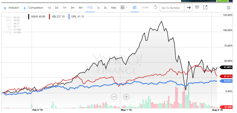
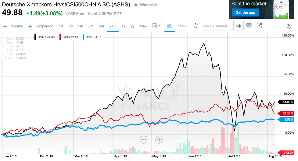
Here is the price graph for these three ETFs from January 1 through August 7th:
How does this graph color your view regarding which investment was “the best” from January 1st through August 7th? If you had been invested in the top performing ETF and you were on blood pressure medicine, would you have been tempted to “up the dose” during June and July, as that ETF tumbled (in almost free fall fashion)? Would being invested in one of the other two ETFs have felt more comfortable, and interfered less frequently with your nightly sleep?
Those of you who keep current on global markets have likely guessed in which sector ETF A invests – Small Cap China A Shares. It is the Deutsche X-Trackers Harvest CSI 500 China ETF (ASHS). To say it has experienced volatility would be a laughable understatement. [To read much more detail about developments in China during the past 8 months, see https://www.markettamer.com/blog/a-free-market-or-macau-with-margin-part-I; and https://www.markettamer.com/blog/a-free-market-or-macau-with-margin-part-ii ).
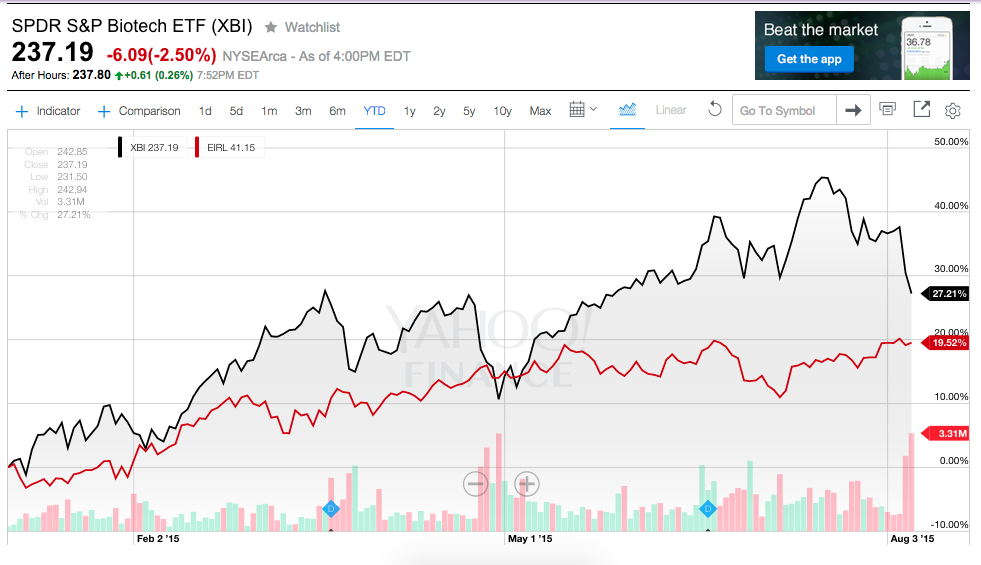
Here is the price graph for ETF B and C:
SPDR S&P Biotech ETF (XBI) has continued to enjoy the multi-year bullish trend in biotech stocks. Although it may have been off your personal radar, the performance of the other ETF — iShares MSCI Ireland Capped (EIRL) – has produced lots of green for investors!
As we have pointed out, both of these ETFs have performed exceptionally – and at a much steadier pace than did ASHS. So we might say we’d be quite content with either investment choice.
But let’s say we were charged with responsibility to suggest to a close friend which of these two ETFs would be a better investment for her/him. What more would we want to know? A list of things we might want to know could include at least the following:
Valuation (Aggregate Price/Earnings Ratio; Price/Sales Ratio; Price/Book Value);
Growth Prospects (Average earnings growth);
Fundamentals (such as prospective economic growth estimates for Ireland);
Analyst opinions regarding intermediate term prospects for Biotech or for Ireland;
Relative Risk
It is that last criteria that I want to focus upon going forward: “Relative Risk”.
I am sure we will all agree that the assessment of “risk” is an essential element in every investment analysis. We sure don’t want to venture into an investment such as ASHS without our eyes wide open to the risks inherent whenever one invests in China – particularly in Small Cap A Shares!! Just imagine how you would feel if you had been invested in ASHS since January, then went on a four-week vacation the evening of June 12 (with ASHS at $76.31/share) and returned on July 7th to find ASHS at just $35.52/share … almost $41 lower!!
Where should we turn to get dependable, rock solid information on Risk — Amanda Drury or Bob Pisani at CNBC; our friendly (high-cost) broker at a major wire house; the pitchman for any given ETF appearing on financial radio or TV; or maybe even our lovable Uncle Wallace[3] from that small town in Kansas?
With all due respect to each of the above persons, I strongly suggest you look elsewhere for counsel on assessing risk. In fact, objective, proven, mathematical measures of risk will be the focus for the rest of this article… following into the next!

A more recent photo of William Sharpe, STANCO 25 Professor Emeritus of Finance at Stanford University’s Graduate School of Business.

William Sharpe many years ago... closer to the days during which he worked on the CAPM and other Valuation Models
William Sharpe[4] is an American economist who, although not nearly as well known as Benjamin Bernanke or Janet Yellen (elevated to international fame through their leadership within the world’s biggest central bank) has undoubtedly had a profound impact upon the investment world. Sharpe literally helped transform the ways that various investments are analyzed.[5] Sharpe was a major force in the vision for and articulation of the “Capital Asset Pricing Model”(CAPM). I addition, he played a key part in the development of the binomial method for the valuation of options, the gradient method for asset allocation optimization, and returns-based style analysis for the evaluation of investment funds. In fact, it might be fair to consider Dr. Sharpe a mathematically oriented investment geek – a geek who won the 1990 Nobel Memorial Prize in Economic Sciences!
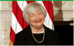
In my opinion, although Fed Chair Yellen is much more widely known than Sharpe, Sharpe has had a much more positive impact upon economics and the investment world.
As you might have guessed from the names of the projects he created or helped shape, they are largely beyond the keen of the average investor (unless well-motivated). But there is one key Sharpe formula that is not only accessible to any investor with a computer and Internet access… but also easily understood and applied in real world investment analysis. That formula is the “Sharpe Ratio”[6] – introduced almost fifty years ago (in 1966).
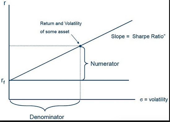
Sharpe’s original intent was to develop a single period forecasting tool that would enable an investor to project how much reward could be expected for investing in a risky asset versus a “risk-free asset” (almost universally assumed to be the 90-Day U.S. Treasury Bill rate). The way Sharpe constructed the formula was both elegant and elementary:
For this formula, these are the component elements:
Return (Rx): any given ETF, fund, or portfolio’s return can be measured for any preferred time interval (daily, weekly, monthly, annually)… as long as said Return is “normally distributed”[7]. A weakness of Sharpe’s formula is that it is not effective with investments that produce asymmetrical returns.[8]
Risk-Free Rate of Return (Rf): this component of the formula enables an investor to discern if she/he is compensated for the incremental risk assumed by investing in a risky asset. [This part of the formula would require much more detail (and likely, some fine print) to satisfy more anal retentive investors (or math geeks). The reason is simple: in an ideal world the Rf chosen in any given calculation would be a “Risk-Free Rate” for a security with a “duration” that matches the duration of the investment with which it is being compared. However, how would one discern the “duration” of ASHS, XBI, or EIRL? And, just as importantly, (all theory aside) in the real world there is no such thing as a totally “Risk-Free Rate” because even the safest investments carry at least a very small amount of risk.] Everyone who has taken high school math or studied Classical Greek Reasoning is familiar with the term “Axiom”[9]. In order to make the Sharpe Ratio a standardized, easily translatable and understood metric… the axiom used in this formula is that the Rf is the then existing rate on 3-Month (90 Day) U.S. Treasury Bills.[10]
Standard Deviation (StdDev): After calculating the excess return (the Return of the asset being analyzed less the Risk-Free Rate) … the final step is to divide the result by the standard deviation of the risky asset being reviewed. [As a reminder, Standard Deviation represents a statistical measurement of dispersion about an average – thereby quantifying how widely an ETF’s (or fund’s or portfolio ‘s) returns varied over a specific period of time.] To help you visualize Standard Deviation, take another look at the graph of ASHS, XBI, and EIRL from January through August 7:
I hope it is obvious that the black line reflects the highest variation in price (therefore, the highest Standard Deviation), the red line has the next highest StdDev and the blue line has the lowest StdDev.
The genius of Sharpe’s formulation is that it allows an objective, quantifiable analysis between two or more ETFs, funds, or portfolios with regard to “Relative Risk”. Indeed, it was the first performance metric that isolated excess return per unit of total risk assumed through any given investment. It has become the “industry standard” for measuring risk-adjusted return… and therefore the metric is much more commonly available to the average investor than are more recent (and often complicated) measures of risk-adjusted return.[11]
Let’s move on to apply what we have learned to the three ETFs with which we started.
I do apologize for the Sharpe Ratio not being available for ASHS due to its nascence. For those who are financially and emotionally prepared to weather the high volatility of the Small Cap China A Shares space, investing a portion of one’s total assets into ASHS may be appropriate.[12] Therefore, to advance our analysis further, let’s compare XBI with EIRL.
I would be thrilled to have owned either XBI or EIRL through August 7th. Once I equip you with one key insight – namely, that a higher Sharpe Ratio[13] indicates that the related ETF (fund or portfolio) generates more return per unit of risk (and therefore offers a higher risk-adjusted return) – you can easily see that EIRL sports a Sharpe Ratio some 24% higher than that of XBI.
I must hasten to add that any given investor may have reasons to prefer XBI over EIRL[14]. But Dr. Sharpe’s work shows us that on a risk-adjusted basis, EIRL definitely offers a higher return!
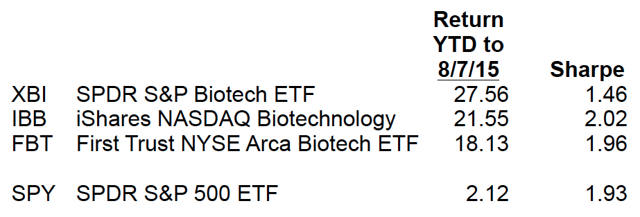
To advance our discussion even further, let’s compare the Sharpe Ratio for three separate popular biotech ETF’s: XBI, iShares NASDAQ Biotechnology (IBB), and First Trust NYSE Arca Biotech ETF (FBT). [I included SPY as a point of reference.]
In this instance, we are not dealing with ETFs from widely divergent investment allocation categories. Instead, we are analyzing three ETFs invested within the biotech space! What can we discern by reviewing the metrics?
First, XBI was far superior on a pure investment return basis – providing shareholders with a return through August 7 that was nearly 28% higher than IBB, and about 52% higher than FBT!
However, according to the Sharpe Ratio, the return that came from XBI was accompanied by a significant degree of additional risk! Therefore, the respective risk-adjusted returns of IBB and FBT (with IBB being slightly higher… and both slightly exceeding that of SPY) are significantly higher (between 34 and 38%) than the risk-adjusted return of XBI.
This does not mean that XBI was a bad investment choice. I can virtually guarantee that no investor whose financial advisor had them in XBI from January through August 7 has called to chew out the advisor for garnering them a return of almost 28% in less than a year!
But it does mean that, on a risk-adjusted basis, IBB and FBT offered a superior return. How any given investor utilizes this industry standard metric is strictly up to that individual.
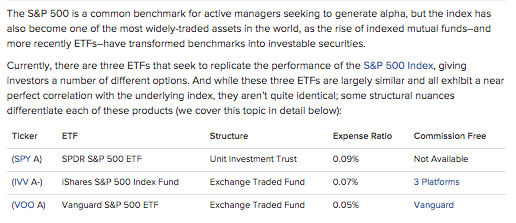
Finally, to provide further context… and confirm (or amplify) a basic tenet of the Sharpe Ratio, let’s compare three big ETFs that purport to offer investors a convenient platform through which to invest (passively) in the S&P 500 Index: SPY, Vanguard S&P 500 ETF (VOO), and iShares Core S&P 500 (IVV). I am not going to post a price chart because, over the 8-month period we are covering, you would be hard pressed to see a difference in the lines. But here is an image of the Sharpe Ratios for SPY, IVV, and VOO:
Trust me – over the course of time, the performance of these three ETFs are equivalent enough that basing an investment decision strictly upon performance or risk-adjusted return could be considered futile.
However, there are aspects of these ETFs that are different, and might offer a prospective investor with objective criteria through which to choose one ETF over another:
As you see, VOO has the lowest annual expense [it is largely for that reason than no less an expert than Warren Buffett has recommended that the trustee for his estate invest 90% of the assets (going to his spouse upon his death) into VOO]. But other ETF costs to consider include bid/ask spreads and transaction commissions. As you see, SPY is not available on a non-commission (or NTF) basis. But IVV is available on that basis through three platforms (you can easily find out which ones), and VOO is commission-free through (of course) Vanguard itself.
INVESTOR TAKEAWAY:
An amazing investment return received over any given time frame will always accrue positively to one’s net worth. However, no investor should neglect being aware of the risk that she/he incurs in exchange for that return. A superb example of the importance of risk assessment is the YTD price graph of ASHS. As we have seen, in less than four weeks it sank by well over 50% (almost $41)! That is what anyone would call a risky investment choice.
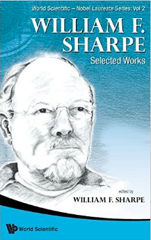
The range of analytical work published by William Sharpe has proven to be a boon to investors since the 1960's.
This is why the Sharpe Ratio is such a boon to investors!
It provides a comprehensible, objective, user-friendly means to measure any given unit of “Return” vis-à-vis the “Risk” that was incurred to realize that return! Expressed more simply, it offers a quick, easy way to calculate one’s “Risk-Adjusted Return” (RAR) … and then compare that RAR with the RAR potentially available through other portfolios, funds, or ETFs.
An obvious corollary of all of the above is the following:
If you have a financial advisor and you have not recently reviewed with said advisor your personal tolerance for risk, I recommend you schedule an appointment soon. During that meeting you might even want to ask the advisor to include the Sharpe Ratio metric to all future investment performance reports. Just don’t tell the advisor that I suggested that!!
DISCLOSURE:
The author does own VOO and owns option positions in SPY. Nothing in this article is intended as a recommendation to buy or sell anything. Always consult with your financial advisor regarding changes in your portfolio – either subtractions or additions.
FOOTNOTES:
[1] Eliminating as well a few very esoteric or thinly traded ETFs.
[2] Standard ETFs for these three performed as follows: GLD (Gold) down almost 8%; JJC (Copper) down almost 19.5%; USO (Oil) down almost 28.5%
[3] Uncle Wallace operates an investment business in his hometown that is located in the furniture store he owns. Oh, and by the way, he is the local funeral director, managing services from the same building.
[4] Born in 1934 (so long past retirement age) Sharpe is the STANCO 25 Professor Emeritus of Finance at Stanford University’s Graduate School of Business.
[5] It should be noted that 50 years from now, Sharpe’s work will likely be found, on balance, to be much more constructive and “accretive” to investment and economic progress than the work of Bernanke and Yellen (who primarily fostered the ballooning of the world’s money supply… the long-term effects of which are potentially staggering.
[6] Full Disclosure: the original name Sharpe gave this formula was “Reward-to-Variability Ratio”. For reasons that will become obvious in moments, the name was soon shortened to the “Sharpe Ratio.”
[7] Note that any normally distributed Return can be easily annualized for analysis.
[8] An example would be certain hedge funds.
[9] From the Greek word axíōma (ἀξίωμα): “that which commends itself as evident.” Or more helpful for you and I in 2015 – “a rule or principle that many people accept as true”
[10] As you know, that rate on August 3rd was 0.08%.
[11] With regard to accessibility, I specifically refer to the metric appearing under the “Risk” link for any given ETF included within YahooFinance.com (assuming of course that the ETF is old enough for them to be able to provide a meaningful, intelligible Sharpe Ratio. For example, of the 11 top performers thus far in 2015, five were not yet “old” enough to have a Sharpe’s Ratio listed. ASHS, for example, is less than a year old.
[12] Quite honestly, I do not personally know anyone in that category.
[13] Except in periods such as 2008-09, during which most equity assets underperformed the Rf… making the Ratio negative… as well as for certain portfolios within which significant leverage is utilized.
[14] They want to be allocated in the Biotech space… they do not want to be invested in the Euro, Europe, or Ireland… etc.
Related Posts
Also on Market Tamer…
Follow Us on Facebook




 Bitcoin, Ethereum, and Dogecoin Soar as “Risk On” Trade Continues